
Master Thesis
Asymptotic Gridshells: applications and analysis
Moaz ABAZA, Pablo FIERRO, Abdel Ghani SAFI, Johan NAVARRO
Abstract
Doubly curved surfaces, among free form surfaces, brought new application opportunities to architecture. These surfaces can be, depending on their principal curvature directions, either synclastic or anticlastic. Usually, because of their principal curves going into the same direction, synclastic surfaces are known to be stable and easier to build. On the other hand, anticlastic surfaces are more challenging to rationalize. In this paper, we will explore the potential of Asymptotic Gridshells and its applications and demonstrate the challenges taken with anticlastic surfaces in construction. This strategy is about matching the property of the materials that can have both bending and torsion, with specific curve properties found on anticlastic surfaces called
Asymptotics. The Pseudocode of finding an Asymptotic curve explained by Eike Schling is coded in a VBscript component for Grasshopper. In this research we apply his algorithm on multiple surfaces in order to compare and analyse the performance of each, with different materials and curvature amount. All surfaces are scaled to approximately 10 to 12 meters long, and the asymptotics of some were compared with the Geodesic gridshell system for being the closer rival system of building anticlastic surfaces. As Asymptotics can be only found on anticlastics, our chosen surfaces vary from completely minimal with 0 constant mean curvature until 0.04 more or less and then are compared. We also investigate the effect of different thicknesses and widths of the planks with the original surface ́s maximum displacement, and stress distribution within the structure. Parametric modeling techniques were used to achieve accurate mathematically built surfaces. Kangaroo 3D developed by Daniel Piker is used for simulation and Form-finding, K2Engineering developed by Cecilie Brandt for structural analysis and load-bearing capacity test in comparison to Karamba3D as they provide both 6DOF structural analysis.
Keywords: Rationalization, Minimal Surface, Anticlastic Surface, Asymptotic GridShell, Active Bending, 6 Degrees of Freedom, K2 Engineering, Karamba3D.
1. Introduction
Asymptotic curves showed great potential when they were applied to a limited number of surfaces. Our research compiles different applications for the understanding of surfaces, design methods, fabrication and construction.
This paper builds on top, to provide a discrete analysis on how this asymptotics gridshells perform on anticlastic surfaces, starting with the interest in the zero mean curvature surfaces, minimal surfaces. This kind of surfaces are those who keep a constant mean curvature along its landscape and are the best scenario for asymptotic directions to show. In minimal surfaces, asymptotic planks intersect at 90 degrees with torsion free nodes and they can be built from planar and straight planks. Other kind of anticlastic that go away from the 0 mean curvature tend to vary in its angle but asymptotics still manage to wrap around properly.

Figure 1: asymptotic gridshell in a catenoid.
As a scope, we will focus on working on different surfaces and compare them from minimal until not so minimal anticlastic surfaces. This will help us to provide the best case study to discover the limits and adaptability strategy.
It is in our deeply interest to add another layer, through new parametric and algorithmic tools, on discovering the proper workflow to calculate the structural stresses, fabrication, assembling and supporting through this specific double curvature surfaces because of how affordable and effective its stripes layout can be, since when unrolled they are flat and straight elements, which makes us save time and money when fabricating.
We want to show the power of these elastic deformation in the materials to rationalise these anticlastic surfaces. Mainly digital modelling specifically 3D parametric algorithmic program Grasshopper for Rhino 6 was used, but we also proved the constructability with some physical mockups.
The digital scripting helps us firstly to take any kind of surface and start by testing if it belongs to the anticlastic type and specifically how much zero mean curvature it has and with the rationalisation through asymptotic curves how feasible is to build.
We oversee simulations and optimize the gridshell in order to facilitate constructability and calculate the load-bearing performance, wind resistance and self weight support.
2. State of the art.
2.1 Synclastic vs Anticlastic

Figure 2: Dome shapes are an example for synclastic surface (left) and saddle like shapes are for anticlastic surface (right).
Synclastic surfaces (left) are known to be easier to build because of its main curvatures going into the same direction. On the opposite, our focus, the anticlastic surfaces (right), have their main curvatures going into opposite directions.
2.2. Asymptotic Curves
Pseudocode explained by Eike Schling in his publication “Designing Grid Structures Using Asymptotic Curve Networks”
In geometry fundamentals:
We can calculate the curvature K for a specific point on a curve with the reciprocal of the radius of the tangent circle.

Figure 3: Curvature K calculation method.
For a point on a surface we can throw curves in all directions and calculate the curvature at the same point.
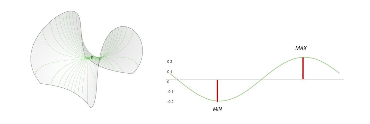
Figure 4: Graph of curvature in 180 Degrees
The resulting graph shows the resulting curvature in 180 degrees pointing, the Max and Min shows the direction of the Principal Curvature lines to calculate K1 and K2 for them.

Figure 5: On the left the resulting Principal Curvature directions, on the right Darboux Frame (Strubecker 1969).
Asymptotics are curves with Kn = 0, with the following equation for calculating Kn in favor of alpha, K1 and K2

Equations 1: Normal plane angle calculation. In consecutive numerical order: (1), (2).
The angle alpha can be calculated to deviate the principal curves to reach the Asymptotic direction as shown in figure 5.

Figure 6: Asymptotic direction deviated from the PC with alpha angle.
The Asymptotic Gridshell is fabricated with planar straight strips of material with no waste, the structure can be assembled flat, all intersections are orthogonal, and the utilization of material is high since it gains more stiffness from the bending and torsion effect. A special case in the anticlastic surfaces family is the Minimal Surface, having a constant 0 mean curvature, which means K1 = K2 and the alpha angle will be 45 degrees. This is translated to a 90 degree intersecting angle in all nodes to simplify the fabrication and load distribution.
2.3. Active bending structures and 6 DOF
As active bending we understand the type of materials, which when bent become stronger because of that elastic deformation.The natural position of the material when bent is trying to go back to its original straight /planar shape.
Six degrees of freedom is the available directions of any body when it moves in a three dimensional space.

Figure 7: 6 DOF of a certain point in 3D space
2.4. Kangaroo by Daniel Piker and K2 Engineering by Cecilie Brandt
Kangaroo is a live physics plugin made for Grasshopper made by Daniel Piker which works for live interactive simulation and form-finding to solve with physical properties the simulation of any wished model to be modified with different parameters and goals.
On the other hand, K2 Engineering is a different plugin for Grasshopper too developed by Cecilie Brandt which is useful to structurally calculate non-linear behaviours in structures (gridshells and cablenets for example). With these software we were able to simulate our chosen surfaces,with the asymptotic gridshells and its bending active materials and behaviours, against wind, point load and other external loads, and calculate its deformation, total amount of stresses and maximum displacements.
2.5. Xavier Tellier's Pre-Rationalisation
The finding of our topic came from the concept of Pre-Rationalisation in a talk given by Xavier Tellier at the UPC. The idea behind it is the feasibility of designing free form architectural shapes but taking into account fabrication and structural efficiency in the form-finding process and generation of the shape.
Xavier states that on any surface, there are peculiar lines that have many useful properties for fabrication. Even though the design of any free form shape might be more constrained, the costs of fabrication can be increasingly lower and even the environmental impact is less.
In our case, the fabrication of asymptotic gridshells completely belongs to pre rationalisation, because before building the gridshell, we focused into anticlastic surfaces only and we cut the surfaces wherever the bounds make construction easier. The main idea about this fabrication is that as we mentioned, when we unroll the asymptotic gridshell, the strips are completely straight, so the material loss can be practically 0, and the nodes will be torsion free.
3. Hypothesis
It is possible to measure how an asymptotic gridshell can perform on anticlastic/minimal surface?
3.1 How far away can we go from a minimal surface?
As one of the objectives of this paper, we will develop a process to measure how an asymptotic gridshell perform on an anticlastic surface and how far can this kind of strategy go away from a minimal surface.
In a more specific way, our study cases will be measured and classified in table of performance to see the proper results by providing a fair scenario of comparison into the scope of our research.
3.2 Boundary cutting
We will see that when unrolled, even most of the minimal surfaces still have a boundary which is not straight when unrolled, which in the case of construction can be a weak point. Starting with the catenoid and going away with other surfaces, we want to see if the shapes can be cut with one of its asymptotic curves, which will make our pieces layout completely straight, feasible to build and can make it even more aesthetic, like our trimmed catenoid.
4. Methodology
4.1. Surface Curvature Analysis
In the look for our research landscape we decided to build a group of surfaces we different kinds of forms and characteristics inside the anticlastic and minimal realm.
As a starting point, we generate a family of anticlastic surfaces through a mathematical cartesian equation or by plugins in which we will be choosing 3, in terms of form, curvature and buildability, to compare these different case studies:

Equations 2: family of equations for anticlastic surfaces. In consecutive numerical order: Catenoid/Helicoid (3), Enneper (class 2) (4), Moebius surface (5), Monkey saddle (6), Henneberg (7), Bour (8). Enneper (class 3) was generated by using the plugin Lunchbox for Grasshopper.

Figure 8: family of surfaces generated. In alphabetical order: Catenoid (a), Enneper (class 3) (b), Enneper (class 2) (c), Moebius surface (d), Monkey saddle (e), Henneberg (f), Bour (g), Helicoid (h).
Once we layout our pool of surfaces, we adapt their geometry and composition by cutting them with an xy plane and controlling their degrees of development in the cartesian cloud of points function definition, also having as a goal an architectural shape with real support points.

Adaptation: we adapt their geometry and composition by cutting them with an xy plane and controlling their degrees of development in the cartesian cloud of points function definition.

Figure 9: family of surfaces generated. In alphabetical order: Catenoid (a), Enneper (class 3) (b), Enneper (class 2) (c), Moebius surface (d), Monkey saddle (e), Henneberg (f), Bour (g), Helicoid (h). The catenoid was deformed to have an option that could perform between our range of research.
Once we have a full family of surface an analysis process is put in place to choose properly our scope.
The first part we analyse the gaussian curvature of the surface in order to see how anticlastic it is. We are going to focus only on the anticlastic surfaces, so any part of the surfaces that shows a gaussian curvature bigger than 0, will not be able to be built with the asymptotics, because of the direction constraints asymptotics curves have. As a maximum value into the gradient we select 0, in order to see the bounds in which each surface perform.
In the second part of the analysis we take a look at the mean curvature. The purpose of this is to determine which surface could give us a fair comparison scenario for the asymptotic curves to be traced. When the surface is completely minimal, the asymptotics in the gridshell will coincide perpendicularly and will have exact perpendicular intersections with torsion free-nodes, resulting in fabrication in straight strips, which obviously makes it more convenient (Eike Schling, 2018).
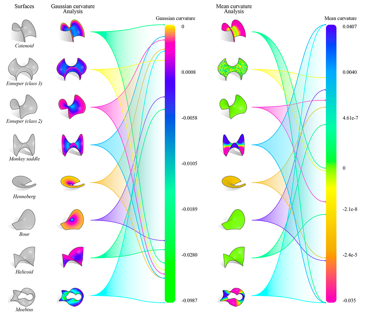
Figure 10: Pool of surfaces analysis of gaussian and mean curvature.
As a result of our analysis, we chose 3 anticlastic surfaces that share a fair measurement in terms of curvature for comparison:
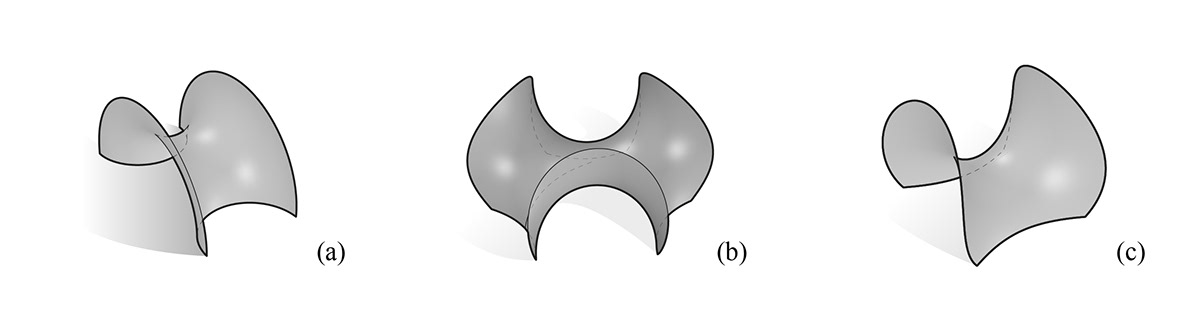
Figure 11: surfaces selected for our analysis scope. Catenoid (a), Enneper (class 3) (b), Enneper (class 2) (c).
4.2 Asymptotic Modeling
Once a surface is cut and finished, an array of points is created along the boundary to generate curves from start points. For the curves to find which path to follow, a VB script requires the surface with a dense grid of uv points for the script to have a proper resolution to find the asymptotics directions on the surface and then calculate the tracing of the curves following it’s vector field.

Figure 12: Asymptotic generation. In the picture: (a) curves direction on surface, (b) asymptotics curves traced on anticlastic surface

Asymptotic curves tracing on a catenoid

Figure 13: Control of the starting point. A crucial aspect to take into account is the position of the points which can result in lines crossing each other (a) in almost the same direction. To have an even spaced grid it’s necessary to optimize the positión of the points carefully (b).
Point positioning for a more equally distance grid
Once we have the polylines of the gridshell traced, the curves are divided into a determined amount of points, and we look for the closest points to the original surface in order to obtain the normals of the surface by evaluating it. We unitized those vectors to have an absolute value and offset the points in order to obtain the lines between the original points and realize the extrusion of the strips.

Figure 14: Asymptotic gridshells generated for analysis. Catenoid (a), Trimmed Catenoid (b), Enneper (class 3) (c), Enneper (class 2) (d).

Once curves are in place, this ones can be extruded by taking the normals of the surface developing the asympotitcs profiles.
4.4 Bearing and bending capacity
With the curves in place, after creating the planes, they will work as an axis to model the asymptotic profiles along the curves. These profiles will provide us the volumes to calculate the different stresses occurring in them. It’s also important to take into consideration its own weight to have a clear bearing capacity measurements.
Our first approach to measure this was through a grasshopper algorithm we created called Analysis Tools where we measure first the torsion and then the bending.

Figure 15: First bending (a) and torsion (b) analysis, measured by degrees per meter.
For the torsion, each polyline is divided into its segments and the torsion between the first and last point of each segment is calculated in a unit we call degrees per meter. For our first surface, the gradient goes from 0.14 to 19.07 degrees per meter having the most torsion in the center of the surface.
In the second part where we measure the bending, we get the perpendicular frames of each segment and we measure the angle between the z vector of the plane and the next one. The results are divided by each segment length, which gives us the final results of degrees of bending per meter. In the case of the catenoid, maximum bending occurs at the edges of the surface, where is less minimal. In order to see the gridshell colours in a smoother way and have more reliable results, we removed three values that were double the maximum of all the other values. We get a maximum of 35.4 degrees per meter at the edges.
As we explained with the previous paragraphs, we got surprising results. We did not know but apparently the torsion and bending are contrary placed in the same surface. Where we had more tension in the surface we had less bending and opposite.
After that algorithm we first made in Grasshopper, we compared those results with the new 6 DOF Plugin for K2 Engineering by Cecilie which we explained in the beginning.
The generation of the file in K2 Engineering was made for each of the chosen surfaces and gridshells.
For the file to work, we needed to have the exact surface and the mesh with the same intersections as the original gridshell in order to generate the planes of how each plank would travel along the surface to then calculate stresses and simulate deformations. The final planes we needed to connect were the cross-product of the perpendicular frames with the normal planes of the surface. With those final planes we created polylines again and then those segments are introduced as bending active into the solver, meaning the relaxed shape of the plank wants to be straight again when bent. With those as beams and its support points, we simulated the gridshell to be working all together with fixed nodes and then displacement of each vertex can be analysed after the simulation, being able to measure stresses as well.
As a result of the algorithm we got the planes (P0,P1), normal forces (N), Shear forces (Vy,Vz), Torsional Moments (Mt), and Bending Moments (My0, My1, Mz0 and Mz1) after the simulation. With those values in each segment and the visualisation display we are able to visualise the bendings My and the torsion in Mt (Mx) changing, depending on the section of planks used.

Figure 16: Planks sections chosen to test each gridshell.
In our case we tried 3 different thicknesses to see the best results for each surface (100 mm, 150 mm and 200 mm) and 4 different widths (6.5mm, 9 mm, 15 mm and 20 mm). The materials taken into account were Birch Plywood, Aluminium and GFRP. The maximum capacities of each material were taken from Engineering Toolbox, from the Handbook of Finnish Plywood and from the website of Nioglas for GFRP in terms of bending and torsion (torsion including shear stresses) and were:
For bending: 35 MPa for wood, 110 MPa for Aluminium and 250 MPa for GFRP, and for torsion the limits were 9.5 MPa for wood, 27 MPa for Aluminium and 60 MPa for GFRP.
Our goal was to calculate all the stresses of all the segments (taking into account only self weight) after the simulation in order to see which sections and which materials work better for each gridshell and the output of 6 Degrees of Freedom does not give those values. In order to get them we extracted the moments about the weak axis and multiplied them with 1e6.With those values in Nmm we calculated each of the section modulus W = (1/6)*b*t^2 = (1/6) * 100 * 10^2 which gave results in mm3. At the end the bending stress as sigma is calculated = M / W for each segment and the result is in MPa.
From all of the bending stresses of each gridshell we took the Maximum bending stress to see if the gridshell would break for bending forces or not.
The other important stresses that were a threat for the gridshell were the moments of torsion and shear that appeared when creating the asymptotic planks. These stresses are actually giving stiffness to the structure when standing. In order to calculate them we use these next formulas. For torsion we first have to calculate MEx (Static Moment) which is the torsional moment and Inertia which depend on the section.
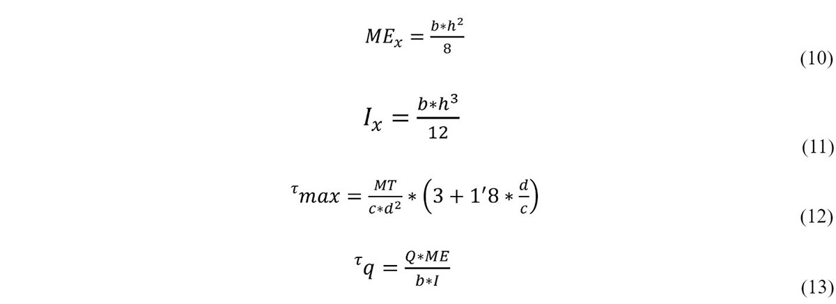
Equations 3: equations of moments present during calculation. In consecutive numerical order: Static moment (10), Inertia moment (11), Torsion(12), Shear (13).
It is important to mention that for Q we used the values from the output of K2E beam that came out as Vz meaning the shear forces for all the segments, and that c was calculated as h (height) and d was calculated as b (base) since the formula of torsion specified that c worked only when it was bigger than d, which is our case.
With these formulas we got these maximum Von Mises for each gridshell. The Von Mises allowed us to have a single number for all the stresses of the plank (bending, torsion, shear) which was the way we could compare all of the gridshells with a single number.
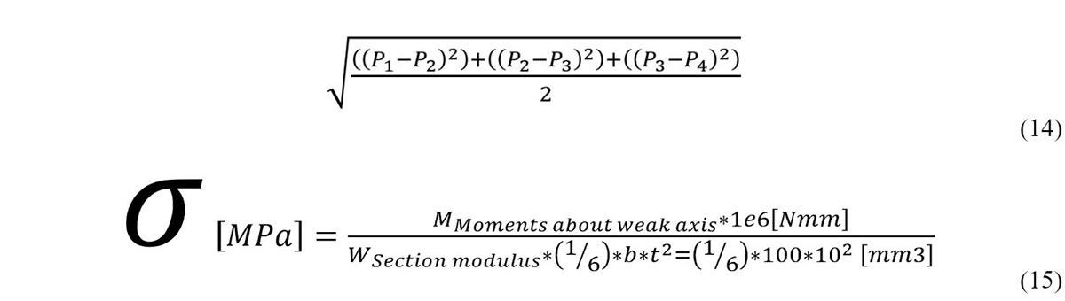
Equations 4: equations of moments present during calculation. In consecutive numerical order: Von Mises (14), Maximum bending stresses (15).
Once we had the scripts working flawlessly, the first thing we realised in K2 Engineering was that our gridshells would need bracing in order to test them against wind. In our parametric script we did animations with wind starting from 0 km/hr t0 100 km/hr, and we were able to know the maximum displacement, maximum von Mises, and with that (knowing the breaking points of each material) the percentage of planks breaking by bending and the ones breaking by torsion at each moment. For bracing in all cases we chose a 15 mm diameter steel cable reinforcing in the main principal curvatures (which was the best proven place to brace).
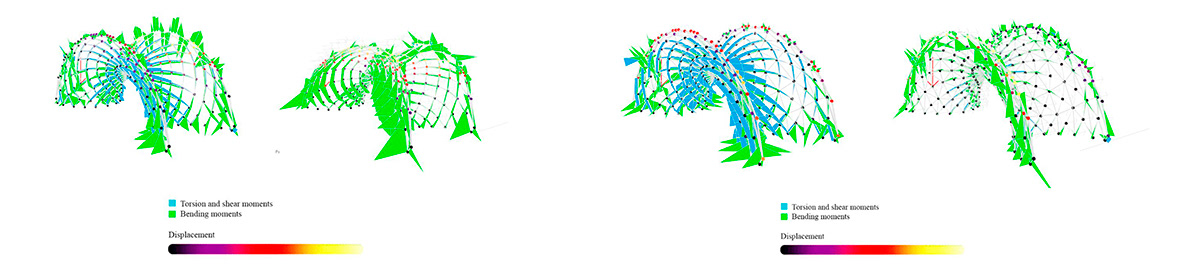
Figure 17 (left): Catenoid deformations without bracing at 0 km/hr (left) and at 100km/hr (right) (with Birch Plywood).
Figure 18 (right): Catenoid deformations with bracing at 0 km/hr (left) and at 100km/hr (right) (with Birch Plywood).
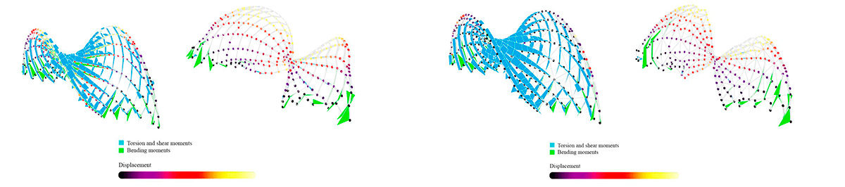
Figure 19 (left): Trimmed catenoid deformations without bracing at 0 km/hr (left) and at 100km/hr (right) (with Birch Plywood).
Figure 20 (right): Trimmed catenoid deformations with bracing at 0 km/hr (left) and at 100km/hr (right) (with Birch Plywood).
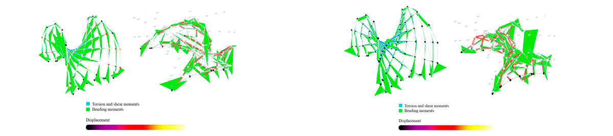
Figure 21 (left): Enneper 2 deformations without bracing at 0 km/hr (left) and at 100km/hr (right) (with Birch Plywood).
Figure 22 (right): Enneper 2 deformations with bracing at 0 km/hr (left) and at 100km/hr (right) (with Birch Plywood).
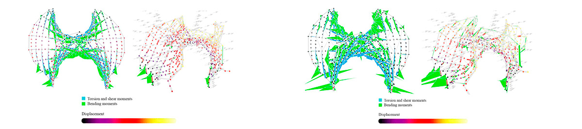
Figure 23 (left): Enneper 2 deformations without bracing at 0 km/hr (left) and at 100km/hr (right) (with Birch Plywood).
Figure 24 (right): Enneper 2 deformations with bracing at 0 km/hr (left) and at 100km/hr (right) (with Birch Plywood).
In terms of utilization, you always want to use the maximum in order to not waste material and take as much advantage of the section you ́re using as possible. In our case, from all of the sections analysed, we decided to choose as the best candidate, the section with less utilisation (meaning the bending stresses were the lowest) in order to test the best sections against wind and external forces. The point of this was to see which section worked better and which material performed best since it's not a linear relationship. We realised that the thickest and the widest planks were not necessarily performing better.
In the following section we show the analysis of utilisation when wind forces are applied to each different gridshell. Each point on the gridshell is representing half of each plank at its boundaries and when converting to red means that part of the plank could not resist and breaks. The script also paints in red the sections that can not resist the stresses. With this script we can analyse the gridshell at any point of the increase of the wind speed and determine how much wind it can resist. In the following images we only show 0 km/hr and 100 km/ hr with birch plywood and without bracing, but in reality we can measure infinite possibilities depending on the scope of the analysis. As an example of how this was measured if a wood plank can resist 35 MPa for bending and in this moment it is using 3.5 MPa, the utilisation in this moment is of 10%.The breaking point is measured when utilisation overpasses 100%.
We know that for security reasons we should never go up to 100% to prevent and stay until 80% for precaution but for this academic purpose that was not taken into account.


Figure 25: Catenoid utilisation without bracing at 0 km/hr (left) and at 100km/hr (right).
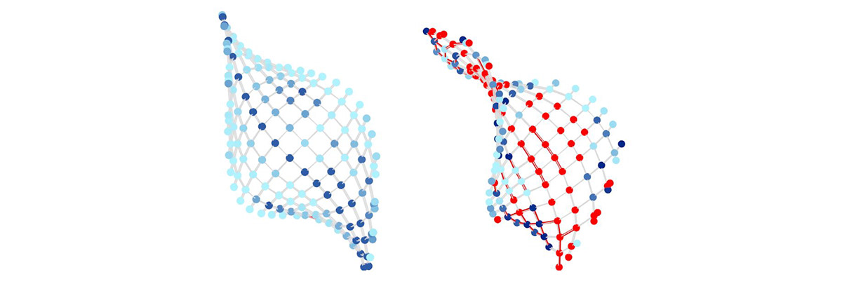
Figure 26: Trimmed catenoid utilisation without bracing at 0 km/hr (left) and at 100km/hr (right).
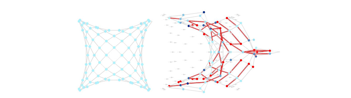
Figure 27: Enneper 2 utilisation without bracing at 0 km/hr (left) and at 100km/hr (right).
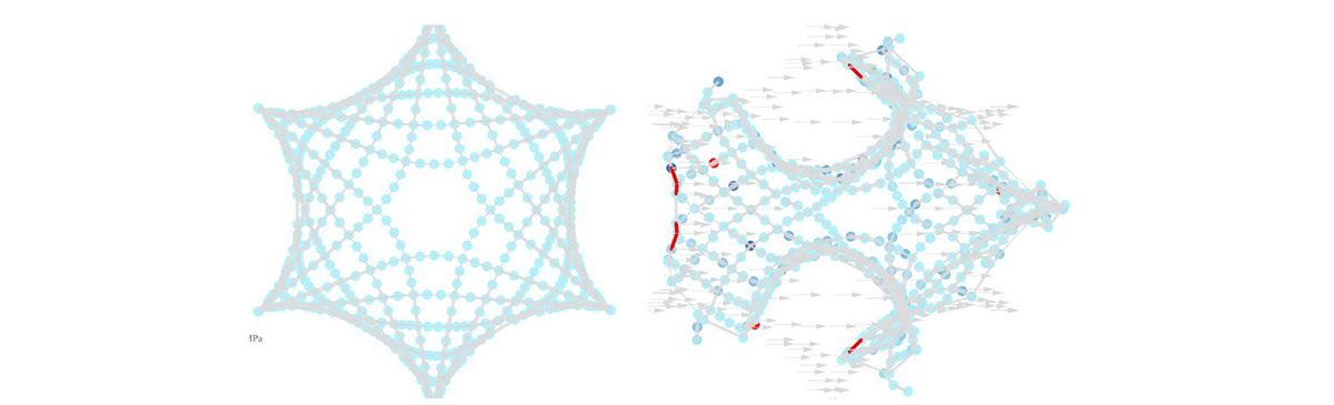
Figure 28: Enneper 3 utilisation without bracing at 0 km/hr (left) and at 100km/hr (right).
After this general analysis of only wood with the same sections measuring utilisation and displacement, we knew we had to focus on the best performing sections of all the ones simulated. That is why the next step was to plot them all in a graph comparing all of the sections in each material, choosing the ones with less Von Mises stresses and less displacement. It is important to mention that in the next graphs we chose a maximum allowable displacement according to the scale that would not affect aesthetics which was 25 cm in a 10 m scale model. We drew a red line and eliminated all the sections that had more displacement than the one we allowed and then the plank section with the less Von Mises stresses was chosen for each gridshell as the graphs below show. We also drew with a red line the maximum Von Mises that the material could handle without breaking in order to only visualize the ones resisting the stresses. In this case only self weight was considered, and the best performing section with less utilisation would be the one candidate to be tested against wind and see the maximum speed it could bear. We also analysed, according with its endurance, which material was having a best percentage of utilisation.

Figure 29: Catenoid structural performance by profile and materials. The best performing section was the 6.5 mm x 100 mm planks ready to be tested against external loads.
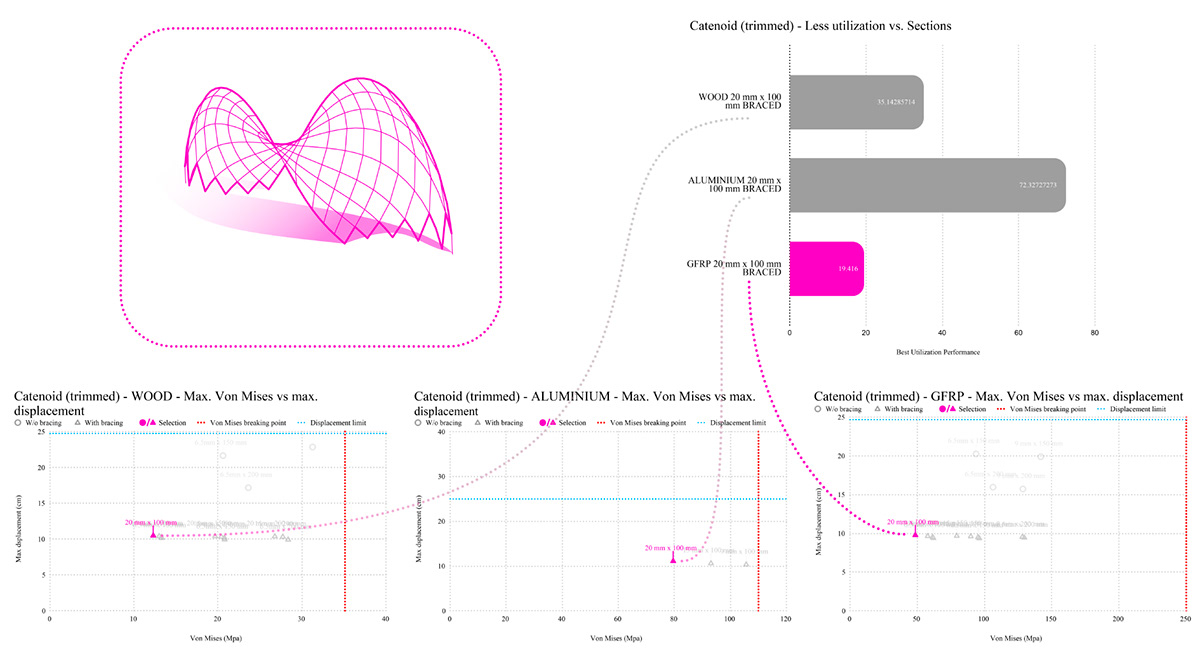
Figure 30: Catenoid (trimmed) structural performance by profile and materials.The best performing section was the mm x 100 mm planks ready to be tested against external loads.

Figure 31: Enneper 2 structural performance by profile and materials. The best performing section was the 6.5 mm x 150 mm planks ready to be tested against external loads.

Figure 32: Enneper 3 structural performance by profile and materials. The best performing section was the 20 mm x 100 mm planks ready to be tested against external loads.
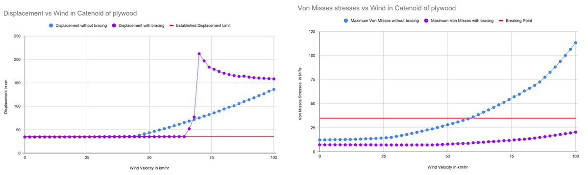
Figure 33: In this graph we show only for the catenoid how bracing vs not braced gridshell behave in terms of wind from 0 to 100 km/hr and how much better bracing works having less Von Mises stress and less displacement.
After knowing which section of planks worked better for each gridshell and having proved that bracing was necessary, we tested each surface with the 3 materials against wind to see the difference in endurance of the materials.
CATENOID

Figure 34: For Birch Plywood with the Catenoid braced the maximum resistance was 117 km/hr. At this point you can see the first 0.9% of the planks overpassing the maximum 35 MPa allowable Von Mises of the wood.

Figure 35: For Aluminium with the Catenoid braced the maximum resistance was 222 km/hr. At this point you can see the first 0.45% of the planks overpassing the maximum 110 MPa allowable Von Mises of the aluminium.

Figure 36: For GFRP with the Catenoid braced the maximum resistance was 282 km/hr. At this point you can see the first 0.45% of the planks overpassing the maximum 250 MPa allowable Von Mises of the GFRP.
Trimmed Catenoid

Figure 37: For Birch Plywood with the Trimmed catenoid braced the maximum resistance was 59 km/hr. At this point you can see the first 0.43% of the planks overpassing the maximum 35 MPa allowable Von Mises of the wood.
Figure 38: For Aluminium with the Trimmed catenoid braced the maximum resistance was 107 km/hr. At this point you can see the first 0.43% of the planks overpassing the maximum 110 MPa allowable Von Mises of the aluminium.

Figure 39: For GFRP with the Trimmed catenoid braced the maximum resistance was 144 km/hr. At this point you can see the first 0.431% of the planks overpassing the maximum 250 MPa allowable Von Mises of the GFRP.
ENNEPER 2

Figure 40: For Birch Plywood with the Enneper 2 braced the maximum resistance was 35 km/hr. At this point you can see the first 0.78% of the planks overpassing the maximum 35 MPa allowable Von Mises of the wood.

Figure 41: For Aluminium with the Enneper 2 braced the maximum resistance was 68 km/hr. At this point you can see the first 0.78125% of the planks overpassing the maximum 110 MPa allowable Von Mises of the aluminium.
Figure 42: For GFRP with the Enneper 2 braced the maximum resistance was 93 km/hr. At this point you can see the first 1.56% of the planks overpassing the maximum 250 MPa allowable Von Mises of the GFRP.
ENNEPER 3
Figure 43: For Birch Plywood with the Enneper 3 braced the maximum resistance was 29 km/hr. At this point you can see the first 0.146% of the planks overpassing the maximum 35 MPa allowable Von Mises of the wood.
Figure 44: For Aluminium with the Enneper 3 braced the maximum resistance was 98 km/hr. At this point you can see the displacement overpassing the established maximum 25 cm allowance.

Figure 45: For GFRP with the Enneper 3 braced the maximum resistance was 30 km/hr. At this point you can see the first 0.44% of the planks overpassing the maximum 250 MPa and the displacement being huge.
4.5 Karamba 3D Shell analysis for bracing

Figure 46: (From left to right) Tension forces, Compression Forces, Force-Flow
Bracing
Once we chose the 3 surfaces to analyze we tested each of them in a structural plugin called Karamba 3D in order to see the principal stress lines in tension, compression and force flow. In the software we analysed each shape as a concrete shell of 25 cm in order to see each surface`s main forces. Based on the surface first, and the stress lines of each, we placed some bracing in order to reinforce stiffness in each gridshell. At the end, after many testings, bracing was placed in the principal curvature lines and analysed as steel cables of 15 mm thickness, where never 2 cables touch each other.
4.4 Flattening the structure
After building the physical model, we realised that the gridshells that could be built from flat, sometimes had bigger stresses when they were flat, since there when they are bent, they want to release that stress and want to be erected by itself.
To be able to calculate those stresses in flat and compare them with the stresses when the gridshells were erected, we used Kangaroo 2 by Daniel Piker setting the main goals to go to the xy plane, line length to be kept as previous, and angle to be zero between the segments, since with bending active materials, when bent, want to go back to the original shape.

Figure 47: Catenoid gridshell erected (left) and in the ground (right).

Figure 48: Catenoid (trimmed) gridshell erected (left) and in the ground (right).

Figure 49: Enneper class 2 erected (left) and in the ground (right).

Figure 50: Enneper class 3 gridshell erected (left) and in the ground (right).


Flattening simulation. From left to right: Catenoid, trimmed catenoid, Enneper 2, Enneper 3
After flattening the structure the results were not straight lines on the xy plane, meaning as we expected that the planks were already bent when flat.
In the following figures we can visualize the bending stresses of each gridshell flat. The interesting part was that the most stress was placed at the boundaries, and when we physically made the models, we realised that it was harder to place them together at the edges as well.
Other interesting finding was the difference in the amount of stress is involved in the non-constant mean surface based gridshell (catenoid and trimmed catenoid) and the mean surface based gridshells (Enneper 2 and 3). Most of the non-constant mean gridshell profiles tested went beyond or close the breaking point, in contrast with the constant mean gridshell in which most of them begun and finish performing inside the boundary of our breaking point.

Figure 51: Catenoid flat stresses behaviour comparison with standing gridshell and standing braced gridshell.

Figure 52: Catenoid (trimmed) flat stresses behaviour comparison with standing gridshell and standing braced gridshell.
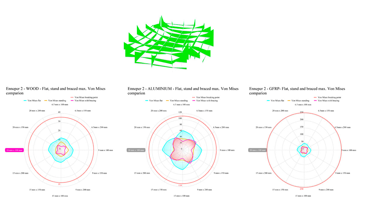
Figure 53: Enneper 2 flat stresses behaviour comparison with standing gridshell and standing braced gridshell.
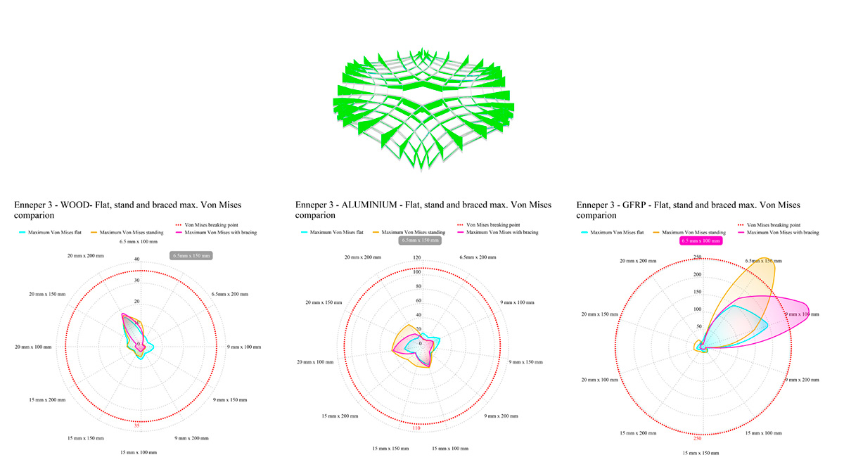
Figure 54: Enneper 3 flat stresses behaviour comparison with standing gridshell and standing braced gridshell.
4.5 Fabrication
Compared with multiple materials, plywood (1mm thickness) has been chosen for its great elastic capacity to build the scaled model. We unrolled the curves and chose the width along with the gap width.


Figure 55: Unroll process
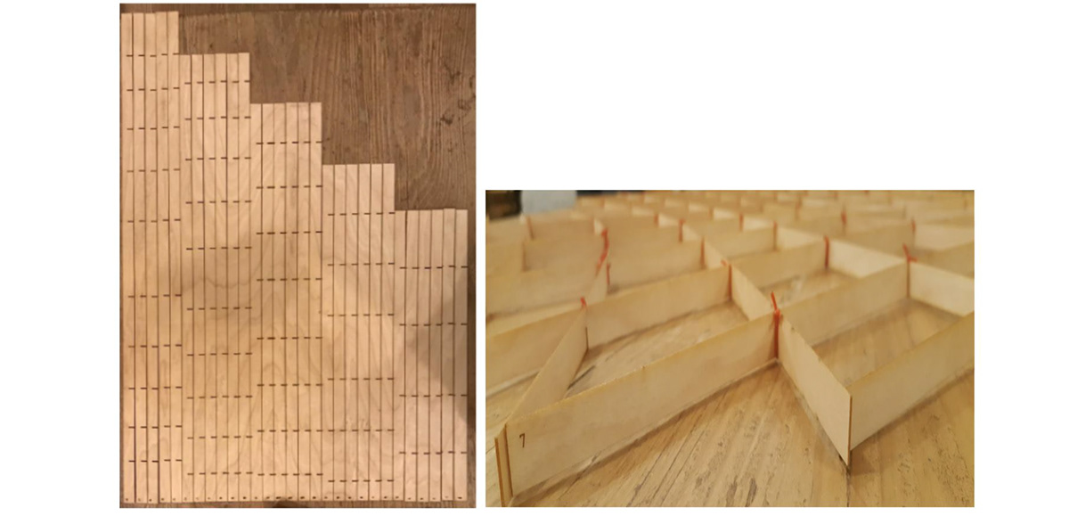
Figure 56: Enneper class 3 model fabrication pieces and nodes connection.
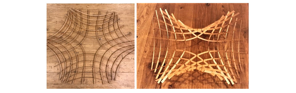
Figure 57: Enneper class 3 model fabrication after and before flattening.
5. Conclusion: submission of contributions
There's nowadays incredible progress in technological fabrication in terms of designing and building freeform surfaces. Historically, every day more, there’s been a liberty of designing new shapes and after Gaudí or Frei Otto the progress with the evolution of computer aided design now we have the capability to analyse more design and fabrication ways. The goal is to subdivide a complicated shape into easy-made parts, in our case flat and straight stripes to avoid material waste and build the gridshell. It is true that we have to accept there are limitations in our shape scope but depending on the shape you want there are different rationalization methods. The goal of our thesis is to make designers aware of the process mentioning and getting deeply into pre-rationalization where the shape can be different from the designer's original proposal but there is still a big scope to choose from. Also all of the minimal surfaces can be cut and rotated and be made more periodic which still increases the possible shapes. In our case we conclude that you can also use any kind of anticlastic surfaces with this rationalisation technique, but sacrificing the 90 degree angle.
To conclude about the gridshells, it always depends on the focus, scale and place you want to build your gridshell in. In this case we just made a comparison of the different possibilities you might encounter when facing this design process.
We realised that stiffness depends a lot about the density of the gridshell and that the inertia of the section is not linear at all. The thicker and the wider the plank is, might not always be the best.
We know you always want to choose the material with more utilization to be able to spend less amount of money and use the more of the section you are paying for. In this research is important to mention that we only focused on the chosen planks using less of the bending resistance (less utilization) to test them against wind and see how much wind (in the worst case scenario) they could bear.
In terms of material, it is more obvious that if you want to build a gridshell 10 meters big and for the exterior, the most suitable material of these 3 might be GFRP because of its bigger stress resistances. But if it's for the interior, maybe with Plywood you will be able to stand more bending stress and more utilisation of the material, so concluding, it totally depends on the focus of the design
The boundary cuts are also a big thing in terms of fabrication. For example, for the catenoid trimmed gridshell, the one we optimised eliminating the curved profiles, we could build it with even the boundaries as straight planks. Summarizing, each case has to be independently analysed because of the complexity of materials, thicknesses and scales that the user needs. As a general comparison we did not find any linear behaviour or relationship between having different sections.
We noticed by comparing the stress in both phases, erected and flat, that some shapes tend to be more relaxed when erected not when flat, which is an interesting point to be researched in the future. After this research we know that if you want to build an asymptotic gridshell you also have to calculate if the planks can resist the bending stresses when the grid is flat on the ground.
Also, the gridshells in this case were tried to be made with homogeneous distances between each plank to have a fair comparison, but we realised that you could also play with having different distances between them, and avoid planks where they are not needed.
5.1 Future Research
- Octopus Evolutionary Optimisation (when target is known)
- Watertight structure ( membrane adding or glass panels)
- Non uniform density grid
- Emu plugin for structural analysis comparison

Figure 58: Planarity Test for each surface for glass panels (left) and membrane geodesic cover (right).
Acknowledgements
We would like to express our special thanks and gratitude to the teachers of the UPC in the Master of Parametric Design in Architecture, who introduced us in this new era and enormous sector of computer designers and brought during the course amazing talks of the most experienced and genius characters in the field like Xavier Tellier, Cecilie Brandt (who was amazingly kind even responding to some doubts about her plugin) and Daniel Piker who are now an example to follow, to Eike Schling who shared his VBscript very gently and obviously to our colleagues who helped us grow together.
References
Eversmann, Philipp; Schling, Eike; Ihde, André; Louter, Christian (2016): Low Cost Double Curvature. Geometrical and Structural Potentials of Rectangular, Cold-bent Glass Construction. In K. Kawaguchi, M. Ohsaki, T. Takeuchi (Eds.): Proceedings of the IASS Annual Symposium 2016. Tokyo.
Schling, Eike; Barthel, Rainer (2017): Experimentelle Studien zur Konstruktion zweifach gekrümmter Gitterstrukturen.Experimental studies on the construction of doubly curved structures: Fachwissen. In Detail structure (01), pp. 52–56.
Schling, Eike; Barthel, Rainer; Tutsch, Joram (2014): Freie Form - experimentelle Tragstruktur. In Bautechnik 91 (12), pp. 859–868.
Schling, Eike; Hitrec, Denis; Barthel, Rainer (2017a): Designing Grid Structures using Asymptotic Curve Networks. In Klaas de Rycke et al. (Eds.): Humanizing Digital Reality. Design Modelling Symposium Paris 2017. Singapore: Springer Singapore, pp. 125–140.
Schling, Eike; Hitrec, Denis; Schikore, Jonas; Barthel, Rainer (2017b): Design and Construction of the Asymptotic Pavilion. In K.-U. Bletzinger,
Eugenio Oñate, B. Kröplin (Eds.): VIII International Conference on Textile Composites and Inflatable Structures. STRUCTURAL MEMBRANES 2017. pp. 178–189.
Schling, Eike; Kilian, Martin; Wang, Hui; Schikore, Jonas; Pottmann, Helmut (2018): Design and Construction of Curved Support Structures with Repetitive Parameters. In Lars Hesselgren, Karl-Gunnar Olsson, Axel Kilian, Samar Malek, Olga Sorkine-Hornung, Chris Williams (Eds.): AAG 2018. Advances in Architectural Geometry. Wien: Klein Publishing, pp. 140–165.
C. Sos Brandt-Olsen, “Calibrated Modelling of Form-active Structures”, Master's thesis in Architectural Engineering, The Technical University of Denmark, June.2016
Engineering ToolBox, (2005). Modulus of Rigidity. [online] Available at: https://www.engineeringtoolbox.com/modulus-rigidity-d_946.html [Accessed 01/08/2019].
Engineering ToolBox, (2003). Young's Modulus - Tensile and Yield Strength for common Materials. [online] Available at:
https://www.engineeringtoolbox.com/young-modulus-d_417.html [Accessed 01/08/2019].
“Handbook of Finnish Plywood”, page 19-20, Koskisen Group, [online] Available at: http://www.koskisen.com
“Mechanical Properties of GFRP”, Nioglas manufactures thermostable polyester-glass fibre profiles, [online] Available at: http://www.nioglas.com/en/propiedades.php
R. Brufau I Niubò, J.R. Blasco I Casanova, “Estructures II Resistència de materials”, Departament D'Estructures A l'Arquitectura.


